Amazon Forecast – Now Generally Available
Getting accurate time series forecasts from historical data is not an easy task. Last year at re:Invent we introduced Amazon Forecast, a fully managed service that requires no experience in machine learning to deliver highly accurate forecasts. I’m excited to share that Amazon Forecast is generally available today!
With Amazon Forecast, there are no servers to provision. You only need to provide historical data, plus any additional metadata that you think may have an impact on your forecasts. For example, the demand for a particular product you need or produce may change with the weather, the time of the year, and the location where the product is used.
Amazon Forecast is based on the same technology used at Amazon and packages our years of experience in building and operating scalable, highly accurate forecasting technology in a way that is easy to use, and can be used for lots of different use cases, such as estimating product demand, cloud computing usage, financial planning, resource planning in a supply chain management system, as it uses deep learning to learn from multiple datasets and automatically try different algorithms.
Using Amazon Forecast
For this post, I need some sample data. To have an interesting use case, I go for the individual household electric power consumption dataset from the UCI Machine Learning Repository. For simplicity, I am using a version where data is aggregated hourly in a file in CSV format. Here are the first few lines where you can see the timestamp, the energy consumption, and the client ID:
2014-01-01 01:00:00,38.34991708126038,client_12
2014-01-01 02:00:00,33.5820895522388,client_12
2014-01-01 03:00:00,34.41127694859037,client_12
2014-01-01 04:00:00,39.800995024875625,client_12
2014-01-01 05:00:00,41.044776119402975,client_12
Let’s see how easy it is to build a predictor and get forecasts by using the Amazon Forecast console. Another option, for more advanced users, would be to use a Jupyter notebook and the AWS SDK for Python. You can find some sample notebooks in this GitHub repository.
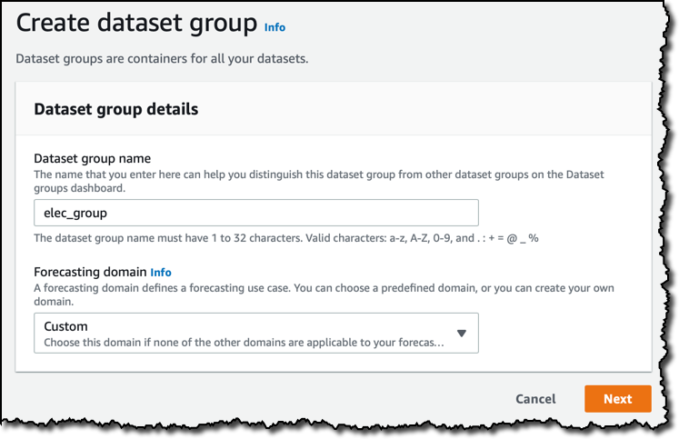
In the Amazon Forecast console, the first step is to create a dataset group. Dataset groups act as containers for datasets that are related.
I can select a forecasting domain for my dataset group. Each domain covers a specific use case, such as retail, inventory planning, or web traffic, and brings its own dataset types based on the type of data used for training. For now, I use a custom domain that covers all use cases that don’t fall in other categories.
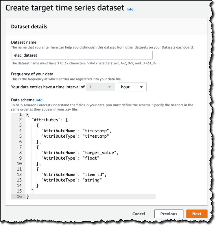
Next, I create a dataset. The data I am going to upload is aggregated by the hour, so 1 hour is the frequency of my data. The default data schema depends on the forecasting domain I selected earlier. I am using a custom domain here, and I change the data schema to have a timestamp, a target_value, and an item_id, in that order, as you can see in the sample few lines of data at the beginning of this post.
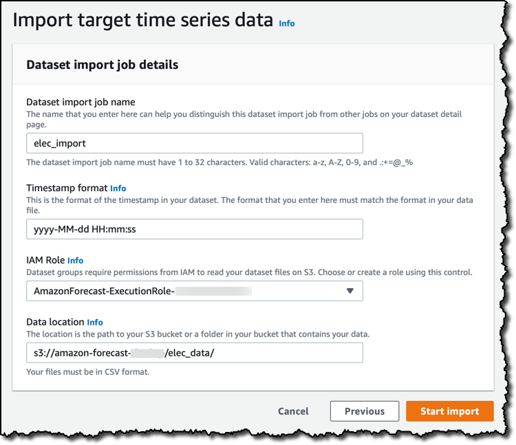
Now is the time to upload my time series data from Amazon Simple Storage Service (S3) into my dataset. The default timestamp format is exactly what I have in my data, so I don’t need to change it. I need an AWS Identity and Access Management (IAM) role to give Amazon Forecast access to the S3 bucket. I can select one here, or create a new one for this use case. As usual, avoid creating IAM roles that are too permissive and apply a least privilege approach to reduce the amount of permissions to the minimum required for this activity. After I tell Amazon Forecast in which S3 bucket and folder to look for my historical data, I start the import job.
The dataset group dashboard gives an overview of the process. My target time series data is being imported, and I can optionally add:
- item metadata information on the items I want to predict on; for example, the color of the items in a retail scenario, or the kind of household (is this an apartment or a detached house?) for this electricity-focused use case.
- related time series data that don’t include the target variable I want to predict, but can help improve my model; for example, price and promotions used by an ecommerce company are probably related to actual sales.
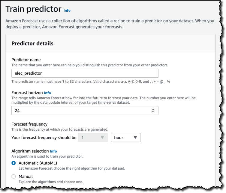
I am not adding more data for this use case. As soon as my dataset is imported, I start to train a predictor that I can then use to generate forecasts. I give the predictor a name, then select the forecast horizon, that in my case is 24 hours, and the frequency at which my forecast are generated.
To train the predictor, I can select a specific machine learning algorithms of my choice, such as ARIMA or DeepAR+, but I prefer simplicity and use AutoML to let Amazon Forecast evaluate all algorithms and choose the one that performs best for my dataset.
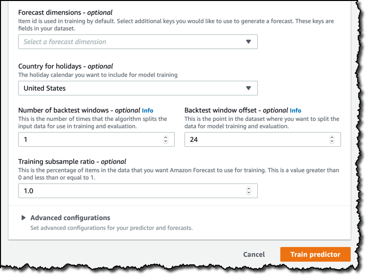
In the case of my dataset, each household is identified by a single variable, the item_id, but you can add more dimensions if required. I can then select the Country for holidays. This is optional, but can improve your results if the data you are using may be affected by people being on holidays or not. I think energy usage is different on holidays, so I select United States, the country my dataset is coming from.
The configuration of the backtest windows is a more advanced topic, and you can skip the next paragraph if you’re not interested into the details of how a machine learning model is evaluated in case of time series. In this case, I am leaving the default.
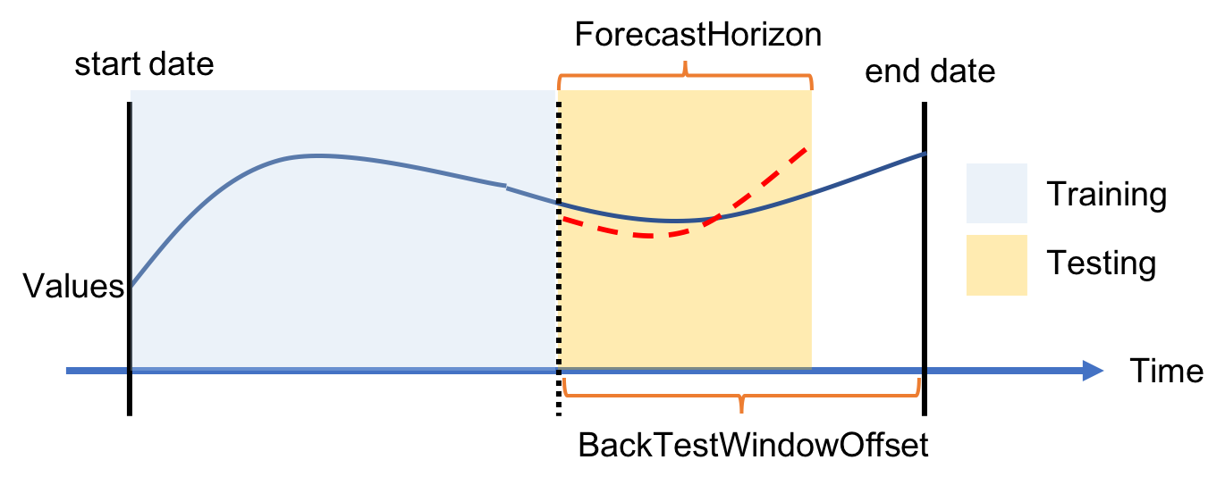
When training a machine learning model, you need two split your dataset in two: a training dataset you use to train with the machine learning algorithm, and an evaluation dataset that you use to evaluate the performance of your trained model. With time series, you can’t just create these two subsets of your data randomly, like you would normally do, because the order of your data points is important. The approach we use for Amazon Forecast is to split the time series in one or more parts, each one called a backtest window, preserving the order of the data. When evaluating your model against a backtest window, you should always use an evaluation dataset of the same length, otherwise it would be very difficult to compare different results. The backtest window offset tells how many points ahead of a split point you want to use for evaluation, and this is the same value for all the splits. For example, by leaving 24 (hours) I always use one day of data for evaluating my model against multiple window offsets.
In the advanced configurations, I have the option to enable hyperparameter optimization (HPO), for the algorithms that support it, and featurizations, to develop additional features computed from the ones in your data. I am not touching those settings now.
After a few minutes, the predictor is active. To understand the quality of a predictor, I look at some of the metrics that are automatically computed.
Quantile loss (QL) calculates how far off the forecast at a certain quantile is from the actual demand. It weights underestimation and overestimation according to a specific quantile. For example, a P90 forecast, if calibrated, means that 90% of the time the true demand is less than the forecast value. Thus, when the demand turns out to be higher than the forecast, the loss would be greater than the other way around.
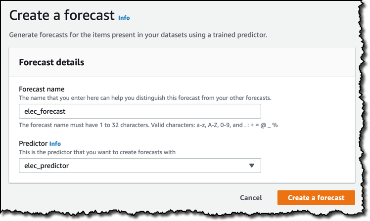
When the predictor is ready, and I am satisfied by its metrics, I can use it to create a forecast.
When the forecast is active, I can query it to get predictions. I can export the whole forecast as CSV file, or query for specific lookups. Let’s do a lookup. In the case of the dataset I am using, I can forecast the energy used by a household for a specific range of time. Dates here are in the past because I used an old dataset. I am pretty sure you’re going to use Amazon Forecast to look into the future.
For each timestamp in the forecast, I get a range of values. The P10, P50, and P90 forecasts have respectively 10%, 50%, and 90% probability of satisfying the actual demand. How you use these three values depends on your use case and how it is impacted by overestimating or underestimating demand. The P50 forecast is the most likely estimate for the demand. The P10 and P90 forecasts give you an 80% confidence interval for what to expect.
Available Now
You can use Amazon Forecast via the console, the AWS Command Line Interface (CLI) and the AWS SDKs. For example, you can use Amazon Forecast within a Jupyter notebook with the AWS SDK for Python to create a new predictor, or use the AWS SDK for JavaScript in the Browser to get predictions from within a web or mobile app, or the AWS SDK for Java or AWS SDK for .NET to add forecast capabilities to an existing enterprise application.
Here’s the overall flow of the Amazon Forecast API, from creating the dataset group to querying and extracting the forecast:
The dataset I used for this walkthrough and other examples are available in this GitHub repository:
Amazon Forecast is now available in US East (N. Virginia), US West (Oregon), US East (Ohio), Europe (Ireland), Asia Pacific (Singapore), and Asia Pacific (Tokyo).
More information on specific features and pricing is one click away at:
I look forward to see what you’re going to use it for, please share your results with me!
— Danilo
Source: AWS News
